For loop

4 minute read

Using loop with R is not the proper behaviour to have. Indeed, using the apply functions family such as tapply, lapply, and so one are a better way to do it, but for me, this is in some case too complicated. The apply family functions improve the speed rate of T and the management of the memory. Thus, apply functions is relevant to use when you have big data-set to play with. Instead of using apply functions, I used for loop. This is simpler to understand it for me and with moderate data-set (about few thousand of rows and 100 columns) the gain of apply functions is limited. Like this, for loop can be read again quickly even when you comeback to your code years later. I will now provide a small example to understand when you can use for loop and how to used them. Also, note that understanding for loop will lead to use foreach function which allow parallelisation computing. It will be explain in another post.

So, let's begin the for loop example. I will show you how to do spaghetti plot from tree ring data.

About the data

Every year, tree make rings. We can count them to have the tree age, and also measure them to know a little more about the tree and its story. Indeed, tree increment (ring width from a year to another) give information on past climate, past disturbances (pest, drought, fire, ice and wind storms, etc.).

In this data set(tree rings increment) you will find tree rings increment [in mm] from 19 different trees (V1 to V19). The NA value is for year without increment information for this tree (it was not born), and the row #270 is for AD 2011 and the row #1 for AD 1741.

The data look like this:

setwd("./assets/data/") # change following your own working directory
library(data.table) #load data.table at least V.1.10 (to have fread function)
increment_data <- fread("tree rings increment.txt")

##if you did not want to use data.table V1.10 (which allow the fread function use the following code
#increment_data <- read.table("tree rings increment.txt",sep=";",h=T) #for your data,
#Because trees have not the same age, there is a lot of NA value and the length of
#your data frame is equal to the year of the oldest trees (for me it was a tree not show in this sub-sample).
#print(increment_data[1:3])

increment_data[, .(V1,V2,V3)]

data.table 1.10.0
  The fastest way to learn (by data.table authors): https://www.datacamp.com/courses/data-analysis-the-data-table-way
  Documentation: ?data.table, example(data.table) and browseVignettes("data.table")
  Release notes, videos and slides: http://r-datatable.com
         V1     V2    V3
  1:     NA     NA    NA
  2:     NA     NA    NA
  3:     NA     NA    NA
  4:     NA     NA    NA
  5:     NA     NA    NA
 ---                    
266: 128.99 182.54 66.89
267: 130.45 182.80 67.14
268: 131.54 183.24 67.50
269: 132.25 183.48 67.73
270: 132.76 184.34 68.14

We are now going to plot each tree starting from their first year of growth record (i.e. the closest year to the row #1), and then continue until the year AD 2011 (i.e. row #270). Because in data-set there is no year with 0 of increment, we need to add it for each trees using the following code example for one tree:

    # the 3 following code line are just to help to generate the graphic frame
increment_data_unique <- increment_data[,1]
increment_data_unique <- increment_data_unique[complete.cases(increment_data_unique) ]
increment_data_unique <- rbind(list(0),increment_data_unique)
# I am pretty sure that those 3 lines of code are not required.
as.data.table(increment_data_unique)

	    V1
     1:   0.00
     2:   0.71
     3:   1.64
     4:   2.07
     5:   2.46
    ---       
   137: 128.99
   138: 130.45
   139: 131.54
   140: 132.25
   141: 132.76

Here we can see that we remove all NA value, and put a 0.00 value for the first year of growth of the tree

Because we need to do it for each 19 trees, this is easier to do it within a for loop like this:

#pdf("Multiplot radial growth sugar maple between 150 and 160 years old.pdf", width=12, height=8) #to save the plot as PDF

plot(as.numeric(rownames(increment_data_unique))-1,increment_data_unique[[1]],xlab="Age [in years]",
     ylab="radial growth [in mm]",main="Radial growth of 19 trees between 150 and 160 yrs",
     type="n",ylim=c(0,250),xlim=c(0,165)) #generate just the frame of the graphic to have all the same scale

for (i in names(increment_data)) { #for loop to draw one by one, each line of tree increments, starting all in age 0
 #use of names(increment_data) to have the names of each trees from "V1" to "V19"

    increment_data_unique <-increment_data[,i,with=F]#with=FALSE to have the whole column
    increment_data_unique <- as.data.frame(increment_data_unique[complete.cases(increment_data_unique), ]) #remove all the NA value
    increment_data_unique <- rbind(0,increment_data_unique) # add the 0 mm of DBH to start all tree at 0 years-old, 0 DBH
    par(new=TRUE) #allow to combine plots
    plot(as.numeric(rownames(increment_data_unique))-1,increment_data_unique[[1]],xlab="Age [in years]",
         ylab="radial growth [in mm]",
         main="Radial growth of 19 trees between 150 and 160 yrs",type="l",ylim=c(0,250),xlim=c(0,165)) #draw the plots for a single tree.
    #then restart the loop with the next tree, etc.
}
#dev.off() # save the graphic in your directory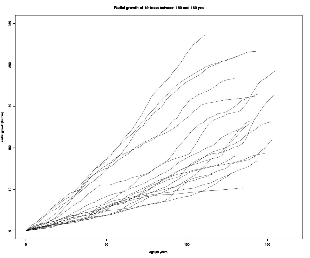

If you want, I have put the all code in my GitHub with the data-set Dendro-spaghetti-plot